> ## Documentation Index
> Fetch the complete documentation index at: https://wb-21fd5541-serverless-sft-revamp.mintlify.site/llms.txt
> Use this file to discover all available pages before exploring further.
# Track models and datasets
export const ColabLink = ({url}) =>
Try in Colab
;
In this notebook, we'll show you how to track your ML experiment pipelines using W\&B Artifacts.
Follow along with a [video tutorial](https://tiny.cc/wb-artifacts-video).
## About artifacts
An artifact, like a Greek [amphora](https://en.wikipedia.org/wiki/Amphora),
is a produced object -- the output of a process.
In ML, the most important artifacts are *datasets* and *models*.
And, like the [Cross of Coronado](https://indianajones.fandom.com/wiki/Cross_of_Coronado), these important artifacts belong in a museum.
That is, they should be cataloged and organized
so that you, your team, and the ML community at large can learn from them.
After all, those who don't track training are doomed to repeat it.
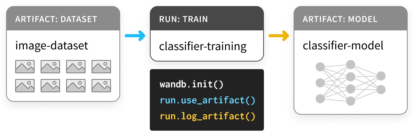
Using our Artifacts API, you can log `Artifact`s as outputs of W\&B `Run`s or use `Artifact`s as input to `Run`s, as in this diagram,
where a training run takes in a dataset and produces a model.
Since one run can use another run's output as an input, `Artifact`s and `Run`s together form a directed graph (a bipartite [DAG](https://en.wikipedia.org/wiki/Directed_acyclic_graph), with nodes for `Artifact`s and `Run`s
and arrows that connect a `Run` to the `Artifact`s it consumes or produces.
## Use artifacts to track models and datatsets
### Install and Import
Artifacts are part of our Python library, starting with version `0.9.2`.
Like most parts of the ML Python stack, it's available via `pip`.
```python theme={null}
# Compatible with wandb version 0.9.2+
!pip install wandb -qqq
!apt install tree
```
```python theme={null}
import os
import wandb
```
### Log a Dataset
First, let's define some Artifacts.
This example is based off of this PyTorch
["Basic MNIST Example"](https://github.com/pytorch/examples/tree/master/mnist/),
but could just as easily have been done in [TensorFlow](https://wandb.me/artifacts-colab), in any other framework,
or in pure Python.
We start with the `Dataset`s:
* a `train`ing set, for choosing the parameters,
* a `validation` set, for choosing the hyperparameters,
* a `test`ing set, for evaluating the final model
The first cell below defines these three datasets.
```python theme={null}
import random
import torch
import torchvision
from torch.utils.data import TensorDataset
from tqdm.auto import tqdm
# Ensure deterministic behavior
torch.backends.cudnn.deterministic = True
random.seed(0)
torch.manual_seed(0)
torch.cuda.manual_seed_all(0)
# Device configuration
device = torch.device("cuda:0" if torch.cuda.is_available() else "cpu")
# Data parameters
num_classes = 10
input_shape = (1, 28, 28)
# drop slow mirror from list of MNIST mirrors
torchvision.datasets.MNIST.mirrors = [mirror for mirror in torchvision.datasets.MNIST.mirrors
if not mirror.startswith("http://yann.lecun.com")]
def load(train_size=50_000):
"""
# Load the data
"""
# the data, split between train and test sets
train = torchvision.datasets.MNIST("./", train=True, download=True)
test = torchvision.datasets.MNIST("./", train=False, download=True)
(x_train, y_train), (x_test, y_test) = (train.data, train.targets), (test.data, test.targets)
# split off a validation set for hyperparameter tuning
x_train, x_val = x_train[:train_size], x_train[train_size:]
y_train, y_val = y_train[:train_size], y_train[train_size:]
training_set = TensorDataset(x_train, y_train)
validation_set = TensorDataset(x_val, y_val)
test_set = TensorDataset(x_test, y_test)
datasets = [training_set, validation_set, test_set]
return datasets
```
This sets up a pattern we'll see repeated in this example:
the code to log the data as an Artifact is wrapped around the code for
producing that data.
In this case, the code for `load`ing the data is
separated out from the code for `load_and_log`ging the data.
This is good practice.
In order to log these datasets as Artifacts,
we just need to
1. create a `Run` with `wandb.init()`, (L4)
2. create an `Artifact` for the dataset (L10), and
3. save and log the associated `file`s (L20, L23).
Check out the example the code cell below
and then expand the sections afterwards for more details.
```python theme={null}
def load_and_log():
# Start a run, with a type to label it and a project it can call home
with wandb.init(project="artifacts-example", job_type="load-data") as run:
datasets = load() # separate code for loading the datasets
names = ["training", "validation", "test"]
# 🏺 create our Artifact
raw_data = wandb.Artifact(
"mnist-raw", type="dataset",
description="Raw MNIST dataset, split into train/val/test",
metadata={"source": "torchvision.datasets.MNIST",
"sizes": [len(dataset) for dataset in datasets]})
for name, data in zip(names, datasets):
# 🐣 Store a new file in the artifact, and write something into its contents.
with raw_data.new_file(name + ".pt", mode="wb") as file:
x, y = data.tensors
torch.save((x, y), file)
# ✍️ Save the artifact to W&B.
run.log_artifact(raw_data)
load_and_log()
```
#### `wandb.init()`
When we make the `Run` that's going to produce the `Artifact`s,
we need to state which `project` it belongs to.
Depending on your workflow,
a project might be as big as `car-that-drives-itself`
or as small as `iterative-architecture-experiment-117`.
> **Best practice**: if you can, keep all of the `Run`s that share `Artifact`s
> inside a single project. This keeps things simple,
> but don't worry -- `Artifact`s are portable across projects.
To help keep track of all the different kinds of jobs you might run,
it's useful to provide a `job_type` when making `Runs`.
This keeps the graph of your Artifacts nice and tidy.
> **Best practice**: the `job_type` should be descriptive and correspond to a single step of your pipeline. Here, we separate out `load`ing data from `preprocess`ing data.
#### `wandb.Artifact`
To log something as an `Artifact`, we have to first make an `Artifact` object.
Every `Artifact` has a `name` -- that's what the first argument sets.
> **Best practice**: the `name` should be descriptive, but easy to remember and type. We like to use names that are hyphen-separated and correspond to variable names in the code.
It also has a `type`. Just like `job_type`s for `Run`s, this is used for organizing the graph of `Run`s and `Artifact`s.
> **Best practice**: the `type` should be simple. Use something more like `dataset` or `model` than `mnist-data-YYYYMMDD`.
You can also attach a `description` and some `metadata`, as a dictionary.
The `metadata` just needs to be serializable to JSON.
> **Best practice**: the `metadata` should be as descriptive as possible.
#### `artifact.new_file` and `run.log_artifact`
Once we've made an `Artifact` object, we need to add files to it.
You read that right: *files* with an *s*.
`Artifact`s are structured like directories,
with files and sub-directories.
> **Best practice**: whenever it makes sense to do so, split the contents
> of an `Artifact` up into multiple files. This will help if it comes time to scale.
We use the `new_file` method
to simultaneously write the file and attach it to the `Artifact`.
Below, we'll use the `add_file` method,
which separates those two steps.
Once we've added all of our files, we need to `log_artifact` to [wandb.ai](https://wandb.ai).
You'll notice some URLs appeared in the output,
including one for the Run page.
That's where you can view the results of the `Run`,
including any `Artifact`s that got logged.
We'll see some examples that make better use of the other components of the Run page below.
### Use a Logged Dataset Artifact
`Artifact`s in W\&B, unlike artifacts in museums,
are designed to be *used*, not just stored.
Let's see what that looks like.
The cell below defines a pipeline step that takes in a raw dataset
and uses it to produce a `preprocess`ed dataset:
`normalize`d and shaped correctly.
Notice again that we split out the meat of the code, `preprocess`,
from the code that interfaces with `wandb`.
```python theme={null}
def preprocess(dataset, normalize=True, expand_dims=True):
"""
## Prepare the data
"""
x, y = dataset.tensors
if normalize:
# Scale images to the [0, 1] range
x = x.type(torch.float32) / 255
if expand_dims:
# Make sure images have shape (1, 28, 28)
x = torch.unsqueeze(x, 1)
return TensorDataset(x, y)
```
Now for the code that instruments this `preprocess` step with `wandb.Artifact` logging.
Note that the example below both `use`s an `Artifact`,
which is new,
and `log`s it,
which is the same as the last step.
`Artifact`s are both the inputs and the outputs of `Run`s.
We use a new `job_type`, `preprocess-data`,
to make it clear that this is a different kind of job from the previous one.
```python theme={null}
def preprocess_and_log(steps):
with wandb.init(project="artifacts-example", job_type="preprocess-data") as run:
processed_data = wandb.Artifact(
"mnist-preprocess", type="dataset",
description="Preprocessed MNIST dataset",
metadata=steps)
# ✔️ declare which artifact we'll be using
raw_data_artifact = run.use_artifact('mnist-raw:latest')
# 📥 if need be, download the artifact
raw_dataset = raw_data_artifact.download()
for split in ["training", "validation", "test"]:
raw_split = read(raw_dataset, split)
processed_dataset = preprocess(raw_split, **steps)
with processed_data.new_file(split + ".pt", mode="wb") as file:
x, y = processed_dataset.tensors
torch.save((x, y), file)
run.log_artifact(processed_data)
def read(data_dir, split):
filename = split + ".pt"
x, y = torch.load(os.path.join(data_dir, filename))
return TensorDataset(x, y)
```
One thing to notice here is that the `steps` of the preprocessing
are saved with the `preprocessed_data` as `metadata`.
If you're trying to make your experiments reproducible,
capturing lots of metadata is a good idea.
Also, even though our dataset is a "`large artifact`",
the `download` step is done in much less than a second.
Expand the markdown cell below for details.
```python theme={null}
steps = {"normalize": True,
"expand_dims": True}
preprocess_and_log(steps)
```
#### `run.use_artifact()`
These steps are simpler. The consumer just needs to know the `name` of the `Artifact`, plus a bit more.
That "bit more" is the `alias` of the particular version of the `Artifact` you want.
By default, the last version to be uploaded is tagged `latest`.
Otherwise, you can pick older versions with `v0`/`v1`, etc.,
or you can provide your own aliases, like `best` or `jit-script`.
Just like [Docker Hub](https://hub.docker.com/) tags,
aliases are separated from names with `:`,
so the `Artifact` we want is `mnist-raw:latest`.
> **Best practice**: Keep aliases short and sweet.
> Use custom `alias`es like `latest` or `best` when you want an `Artifact`
> that satisifies some property
#### `artifact.download`
Now, you may be worrying about the `download` call.
If we download another copy, won't that double the burden on memory?
Don't worry friend. Before we actually download anything,
we check to see if the right version is available locally.
This uses the same technology that underlies [torrenting](https://en.wikipedia.org/wiki/Torrent_file) and [version control with `git`](https://blog.thoughtram.io/git/2014/11/18/the-anatomy-of-a-git-commit.html): hashing.
As `Artifact`s are created and logged,
a folder called `artifacts` in the working directory
will start to fill with sub-directories,
one for each `Artifact`.
Check out its contents with `!tree artifacts`:
```python theme={null}
!tree artifacts
```
#### The Artifacts page
Now that we've logged and used an `Artifact`,
let's check out the Artifacts tab on the Run page.
Navigate to the Run page URL from the `wandb` output
and select the "Artifacts" tab from the left sidebar
(it's the one with the database icon,
which looks like three hockey pucks stacked on top of one another).
Click a row in either the **Input Artifacts** table
or in the **Output Artifacts** table,
then check out the tabs (**Overview**, **Metadata**)
to see everything logged about the `Artifact`.
We particularly like the **Graph View**.
By default, it shows a graph
with the `type`s of `Artifact`s
and the `job_type`s of `Run` as the two types of nodes,
with arrows to represent consumption and production.
### Log a Model
That's enough to see how the API for `Artifact`s works,
but let's follow this example through to the end of the pipeline
so we can see how `Artifact`s can improve your ML workflow.
This first cell here builds a DNN `model` in PyTorch -- a really simple ConvNet.
We'll start by just initializing the `model`, not training it.
That way, we can repeat the training while keeping everything else constant.
```python theme={null}
from math import floor
import torch.nn as nn
class ConvNet(nn.Module):
def __init__(self, hidden_layer_sizes=[32, 64],
kernel_sizes=[3],
activation="ReLU",
pool_sizes=[2],
dropout=0.5,
num_classes=num_classes,
input_shape=input_shape):
super(ConvNet, self).__init__()
self.layer1 = nn.Sequential(
nn.Conv2d(in_channels=input_shape[0], out_channels=hidden_layer_sizes[0], kernel_size=kernel_sizes[0]),
getattr(nn, activation)(),
nn.MaxPool2d(kernel_size=pool_sizes[0])
)
self.layer2 = nn.Sequential(
nn.Conv2d(in_channels=hidden_layer_sizes[0], out_channels=hidden_layer_sizes[-1], kernel_size=kernel_sizes[-1]),
getattr(nn, activation)(),
nn.MaxPool2d(kernel_size=pool_sizes[-1])
)
self.layer3 = nn.Sequential(
nn.Flatten(),
nn.Dropout(dropout)
)
fc_input_dims = floor((input_shape[1] - kernel_sizes[0] + 1) / pool_sizes[0]) # layer 1 output size
fc_input_dims = floor((fc_input_dims - kernel_sizes[-1] + 1) / pool_sizes[-1]) # layer 2 output size
fc_input_dims = fc_input_dims*fc_input_dims*hidden_layer_sizes[-1] # layer 3 output size
self.fc = nn.Linear(fc_input_dims, num_classes)
def forward(self, x):
x = self.layer1(x)
x = self.layer2(x)
x = self.layer3(x)
x = self.fc(x)
return x
```
Here, we're using W\&B to track the run,
and so using the [`run.config`](https://colab.research.google.com/github/wandb/examples/blob/master/colabs/wandb-config/Configs_in_W%26B.ipynb)
object to store all of the hyperparameters.
The `dict`ionary version of that `config` object is a really useful piece of `metadata`, so make sure to include it.
```python theme={null}
def build_model_and_log(config):
with wandb.init(project="artifacts-example", job_type="initialize", config=config) as run:
config = run.config
model = ConvNet(**config)
model_artifact = wandb.Artifact(
"convnet", type="model",
description="Simple AlexNet style CNN",
metadata=dict(config))
torch.save(model.state_dict(), "initialized_model.pth")
# ➕ another way to add a file to an Artifact
model_artifact.add_file("initialized_model.pth")
run.save("initialized_model.pth")
run.log_artifact(model_artifact)
model_config = {"hidden_layer_sizes": [32, 64],
"kernel_sizes": [3],
"activation": "ReLU",
"pool_sizes": [2],
"dropout": 0.5,
"num_classes": 10}
build_model_and_log(model_config)
```
#### `artifact.add_file()`
Instead of simultaneously writing a `new_file` and adding it to the `Artifact`,
as in the dataset logging examples,
we can also write files in one step
(here, `torch.save`)
and then `add` them to the `Artifact` in another.
> **Best practice**: use `new_file` when you can, to prevent duplication.
#### Use a Logged Model Artifact
Just like we could call `use_artifact` on a `dataset`,
we can call it on our `initialized_model`
to use it in another `Run`.
This time, let's `train` the `model`.
For more details, check out our Colab on
[instrumenting W\&B with PyTorch](https://wandb.me/pytorch-colab).
```python theme={null}
import wandb
import torch.nn.functional as F
def train(model, train_loader, valid_loader, config):
optimizer = getattr(torch.optim, config.optimizer)(model.parameters())
model.train()
example_ct = 0
for epoch in range(config.epochs):
for batch_idx, (data, target) in enumerate(train_loader):
data, target = data.to(device), target.to(device)
optimizer.zero_grad()
output = model(data)
loss = F.cross_entropy(output, target)
loss.backward()
optimizer.step()
example_ct += len(data)
if batch_idx % config.batch_log_interval == 0:
print('Train Epoch: {} [{}/{} ({:.0%})]\tLoss: {:.6f}'.format(
epoch, batch_idx * len(data), len(train_loader.dataset),
batch_idx / len(train_loader), loss.item()))
train_log(loss, example_ct, epoch)
# evaluate the model on the validation set at each epoch
loss, accuracy = test(model, valid_loader)
test_log(loss, accuracy, example_ct, epoch)
def test(model, test_loader):
model.eval()
test_loss = 0
correct = 0
with torch.no_grad():
for data, target in test_loader:
data, target = data.to(device), target.to(device)
output = model(data)
test_loss += F.cross_entropy(output, target, reduction='sum') # sum up batch loss
pred = output.argmax(dim=1, keepdim=True) # get the index of the max log-probability
correct += pred.eq(target.view_as(pred)).sum()
test_loss /= len(test_loader.dataset)
accuracy = 100. * correct / len(test_loader.dataset)
return test_loss, accuracy
def train_log(loss, example_ct, epoch):
loss = float(loss)
# where the magic happens
with wandb.init(project="artifacts-example", job_type="train") as run:
run.log({"epoch": epoch, "train/loss": loss}, step=example_ct)
print(f"Loss after " + str(example_ct).zfill(5) + f" examples: {loss:.3f}")
def test_log(loss, accuracy, example_ct, epoch):
loss = float(loss)
accuracy = float(accuracy)
# where the magic happens
with wandb.init() as run:
run.log({"epoch": epoch, "validation/loss": loss, "validation/accuracy": accuracy}, step=example_ct)
print(f"Loss/accuracy after " + str(example_ct).zfill(5) + f" examples: {loss:.3f}/{accuracy:.3f}")
```
We'll run two separate `Artifact`-producing `Run`s this time.
Once the first finishes `train`ing the `model`,
the `second` will consume the `trained-model` `Artifact`
by `evaluate`ing its performance on the `test_dataset`.
Also, we'll pull out the 32 examples on which the network gets the most confused --
on which the `categorical_crossentropy` is highest.
This is a good way to diagnose issues with your dataset and your model.
```python theme={null}
def evaluate(model, test_loader):
"""
## Evaluate the trained model
"""
loss, accuracy = test(model, test_loader)
highest_losses, hardest_examples, true_labels, predictions = get_hardest_k_examples(model, test_loader.dataset)
return loss, accuracy, highest_losses, hardest_examples, true_labels, predictions
def get_hardest_k_examples(model, testing_set, k=32):
model.eval()
loader = DataLoader(testing_set, 1, shuffle=False)
# get the losses and predictions for each item in the dataset
losses = None
predictions = None
with torch.no_grad():
for data, target in loader:
data, target = data.to(device), target.to(device)
output = model(data)
loss = F.cross_entropy(output, target)
pred = output.argmax(dim=1, keepdim=True)
if losses is None:
losses = loss.view((1, 1))
predictions = pred
else:
losses = torch.cat((losses, loss.view((1, 1))), 0)
predictions = torch.cat((predictions, pred), 0)
argsort_loss = torch.argsort(losses, dim=0)
highest_k_losses = losses[argsort_loss[-k:]]
hardest_k_examples = testing_set[argsort_loss[-k:]][0]
true_labels = testing_set[argsort_loss[-k:]][1]
predicted_labels = predictions[argsort_loss[-k:]]
return highest_k_losses, hardest_k_examples, true_labels, predicted_labels
```
These logging functions don't add any new `Artifact` features,
so we won't comment on them:
we're just `use`ing, `download`ing,
and `log`ging `Artifact`s.
```python theme={null}
from torch.utils.data import DataLoader
def train_and_log(config):
with wandb.init(project="artifacts-example", job_type="train", config=config) as run:
config = run.config
data = run.use_artifact('mnist-preprocess:latest')
data_dir = data.download()
training_dataset = read(data_dir, "training")
validation_dataset = read(data_dir, "validation")
train_loader = DataLoader(training_dataset, batch_size=config.batch_size)
validation_loader = DataLoader(validation_dataset, batch_size=config.batch_size)
model_artifact = run.use_artifact("convnet:latest")
model_dir = model_artifact.download()
model_path = os.path.join(model_dir, "initialized_model.pth")
model_config = model_artifact.metadata
config.update(model_config)
model = ConvNet(**model_config)
model.load_state_dict(torch.load(model_path))
model = model.to(device)
train(model, train_loader, validation_loader, config)
model_artifact = wandb.Artifact(
"trained-model", type="model",
description="Trained NN model",
metadata=dict(model_config))
torch.save(model.state_dict(), "trained_model.pth")
model_artifact.add_file("trained_model.pth")
run.save("trained_model.pth")
run.log_artifact(model_artifact)
return model
def evaluate_and_log(config=None):
with wandb.init(project="artifacts-example", job_type="report", config=config) as run:
data = run.use_artifact('mnist-preprocess:latest')
data_dir = data.download()
testing_set = read(data_dir, "test")
test_loader = torch.utils.data.DataLoader(testing_set, batch_size=128, shuffle=False)
model_artifact = run.use_artifact("trained-model:latest")
model_dir = model_artifact.download()
model_path = os.path.join(model_dir, "trained_model.pth")
model_config = model_artifact.metadata
model = ConvNet(**model_config)
model.load_state_dict(torch.load(model_path))
model.to(device)
loss, accuracy, highest_losses, hardest_examples, true_labels, preds = evaluate(model, test_loader)
run.summary.update({"loss": loss, "accuracy": accuracy})
run.log({"high-loss-examples":
[wandb.Image(hard_example, caption=str(int(pred)) + "," + str(int(label)))
for hard_example, pred, label in zip(hardest_examples, preds, true_labels)]})
```
```python theme={null}
train_config = {"batch_size": 128,
"epochs": 5,
"batch_log_interval": 25,
"optimizer": "Adam"}
model = train_and_log(train_config)
evaluate_and_log()
```
 Since one run can use another run's output as an input, `Artifact`s and `Run`s together form a directed graph (a bipartite [DAG](https://en.wikipedia.org/wiki/Directed_acyclic_graph), with nodes for `Artifact`s and `Run`s
and arrows that connect a `Run` to the `Artifact`s it consumes or produces.
## Use artifacts to track models and datatsets
### Install and Import
Artifacts are part of our Python library, starting with version `0.9.2`.
Like most parts of the ML Python stack, it's available via `pip`.
```python theme={null}
# Compatible with wandb version 0.9.2+
!pip install wandb -qqq
!apt install tree
```
```python theme={null}
import os
import wandb
```
### Log a Dataset
First, let's define some Artifacts.
This example is based off of this PyTorch
["Basic MNIST Example"](https://github.com/pytorch/examples/tree/master/mnist/),
but could just as easily have been done in [TensorFlow](https://wandb.me/artifacts-colab), in any other framework,
or in pure Python.
We start with the `Dataset`s:
* a `train`ing set, for choosing the parameters,
* a `validation` set, for choosing the hyperparameters,
* a `test`ing set, for evaluating the final model
The first cell below defines these three datasets.
```python theme={null}
import random
import torch
import torchvision
from torch.utils.data import TensorDataset
from tqdm.auto import tqdm
# Ensure deterministic behavior
torch.backends.cudnn.deterministic = True
random.seed(0)
torch.manual_seed(0)
torch.cuda.manual_seed_all(0)
# Device configuration
device = torch.device("cuda:0" if torch.cuda.is_available() else "cpu")
# Data parameters
num_classes = 10
input_shape = (1, 28, 28)
# drop slow mirror from list of MNIST mirrors
torchvision.datasets.MNIST.mirrors = [mirror for mirror in torchvision.datasets.MNIST.mirrors
if not mirror.startswith("http://yann.lecun.com")]
def load(train_size=50_000):
"""
# Load the data
"""
# the data, split between train and test sets
train = torchvision.datasets.MNIST("./", train=True, download=True)
test = torchvision.datasets.MNIST("./", train=False, download=True)
(x_train, y_train), (x_test, y_test) = (train.data, train.targets), (test.data, test.targets)
# split off a validation set for hyperparameter tuning
x_train, x_val = x_train[:train_size], x_train[train_size:]
y_train, y_val = y_train[:train_size], y_train[train_size:]
training_set = TensorDataset(x_train, y_train)
validation_set = TensorDataset(x_val, y_val)
test_set = TensorDataset(x_test, y_test)
datasets = [training_set, validation_set, test_set]
return datasets
```
This sets up a pattern we'll see repeated in this example:
the code to log the data as an Artifact is wrapped around the code for
producing that data.
In this case, the code for `load`ing the data is
separated out from the code for `load_and_log`ging the data.
This is good practice.
In order to log these datasets as Artifacts,
we just need to
1. create a `Run` with `wandb.init()`, (L4)
2. create an `Artifact` for the dataset (L10), and
3. save and log the associated `file`s (L20, L23).
Check out the example the code cell below
and then expand the sections afterwards for more details.
```python theme={null}
def load_and_log():
# Start a run, with a type to label it and a project it can call home
with wandb.init(project="artifacts-example", job_type="load-data") as run:
datasets = load() # separate code for loading the datasets
names = ["training", "validation", "test"]
# 🏺 create our Artifact
raw_data = wandb.Artifact(
"mnist-raw", type="dataset",
description="Raw MNIST dataset, split into train/val/test",
metadata={"source": "torchvision.datasets.MNIST",
"sizes": [len(dataset) for dataset in datasets]})
for name, data in zip(names, datasets):
# 🐣 Store a new file in the artifact, and write something into its contents.
with raw_data.new_file(name + ".pt", mode="wb") as file:
x, y = data.tensors
torch.save((x, y), file)
# ✍️ Save the artifact to W&B.
run.log_artifact(raw_data)
load_and_log()
```
#### `wandb.init()`
When we make the `Run` that's going to produce the `Artifact`s,
we need to state which `project` it belongs to.
Depending on your workflow,
a project might be as big as `car-that-drives-itself`
or as small as `iterative-architecture-experiment-117`.
> **Best practice**: if you can, keep all of the `Run`s that share `Artifact`s
> inside a single project. This keeps things simple,
> but don't worry -- `Artifact`s are portable across projects.
To help keep track of all the different kinds of jobs you might run,
it's useful to provide a `job_type` when making `Runs`.
This keeps the graph of your Artifacts nice and tidy.
> **Best practice**: the `job_type` should be descriptive and correspond to a single step of your pipeline. Here, we separate out `load`ing data from `preprocess`ing data.
#### `wandb.Artifact`
To log something as an `Artifact`, we have to first make an `Artifact` object.
Every `Artifact` has a `name` -- that's what the first argument sets.
> **Best practice**: the `name` should be descriptive, but easy to remember and type. We like to use names that are hyphen-separated and correspond to variable names in the code.
It also has a `type`. Just like `job_type`s for `Run`s, this is used for organizing the graph of `Run`s and `Artifact`s.
> **Best practice**: the `type` should be simple. Use something more like `dataset` or `model` than `mnist-data-YYYYMMDD`.
You can also attach a `description` and some `metadata`, as a dictionary.
The `metadata` just needs to be serializable to JSON.
> **Best practice**: the `metadata` should be as descriptive as possible.
#### `artifact.new_file` and `run.log_artifact`
Once we've made an `Artifact` object, we need to add files to it.
You read that right: *files* with an *s*.
`Artifact`s are structured like directories,
with files and sub-directories.
> **Best practice**: whenever it makes sense to do so, split the contents
> of an `Artifact` up into multiple files. This will help if it comes time to scale.
We use the `new_file` method
to simultaneously write the file and attach it to the `Artifact`.
Below, we'll use the `add_file` method,
which separates those two steps.
Once we've added all of our files, we need to `log_artifact` to [wandb.ai](https://wandb.ai).
You'll notice some URLs appeared in the output,
including one for the Run page.
That's where you can view the results of the `Run`,
including any `Artifact`s that got logged.
We'll see some examples that make better use of the other components of the Run page below.
### Use a Logged Dataset Artifact
`Artifact`s in W\&B, unlike artifacts in museums,
are designed to be *used*, not just stored.
Let's see what that looks like.
The cell below defines a pipeline step that takes in a raw dataset
and uses it to produce a `preprocess`ed dataset:
`normalize`d and shaped correctly.
Notice again that we split out the meat of the code, `preprocess`,
from the code that interfaces with `wandb`.
```python theme={null}
def preprocess(dataset, normalize=True, expand_dims=True):
"""
## Prepare the data
"""
x, y = dataset.tensors
if normalize:
# Scale images to the [0, 1] range
x = x.type(torch.float32) / 255
if expand_dims:
# Make sure images have shape (1, 28, 28)
x = torch.unsqueeze(x, 1)
return TensorDataset(x, y)
```
Now for the code that instruments this `preprocess` step with `wandb.Artifact` logging.
Note that the example below both `use`s an `Artifact`,
which is new,
and `log`s it,
which is the same as the last step.
`Artifact`s are both the inputs and the outputs of `Run`s.
We use a new `job_type`, `preprocess-data`,
to make it clear that this is a different kind of job from the previous one.
```python theme={null}
def preprocess_and_log(steps):
with wandb.init(project="artifacts-example", job_type="preprocess-data") as run:
processed_data = wandb.Artifact(
"mnist-preprocess", type="dataset",
description="Preprocessed MNIST dataset",
metadata=steps)
# ✔️ declare which artifact we'll be using
raw_data_artifact = run.use_artifact('mnist-raw:latest')
# 📥 if need be, download the artifact
raw_dataset = raw_data_artifact.download()
for split in ["training", "validation", "test"]:
raw_split = read(raw_dataset, split)
processed_dataset = preprocess(raw_split, **steps)
with processed_data.new_file(split + ".pt", mode="wb") as file:
x, y = processed_dataset.tensors
torch.save((x, y), file)
run.log_artifact(processed_data)
def read(data_dir, split):
filename = split + ".pt"
x, y = torch.load(os.path.join(data_dir, filename))
return TensorDataset(x, y)
```
One thing to notice here is that the `steps` of the preprocessing
are saved with the `preprocessed_data` as `metadata`.
If you're trying to make your experiments reproducible,
capturing lots of metadata is a good idea.
Also, even though our dataset is a "`large artifact`",
the `download` step is done in much less than a second.
Expand the markdown cell below for details.
```python theme={null}
steps = {"normalize": True,
"expand_dims": True}
preprocess_and_log(steps)
```
#### `run.use_artifact()`
These steps are simpler. The consumer just needs to know the `name` of the `Artifact`, plus a bit more.
That "bit more" is the `alias` of the particular version of the `Artifact` you want.
By default, the last version to be uploaded is tagged `latest`.
Otherwise, you can pick older versions with `v0`/`v1`, etc.,
or you can provide your own aliases, like `best` or `jit-script`.
Just like [Docker Hub](https://hub.docker.com/) tags,
aliases are separated from names with `:`,
so the `Artifact` we want is `mnist-raw:latest`.
> **Best practice**: Keep aliases short and sweet.
> Use custom `alias`es like `latest` or `best` when you want an `Artifact`
> that satisifies some property
#### `artifact.download`
Now, you may be worrying about the `download` call.
If we download another copy, won't that double the burden on memory?
Don't worry friend. Before we actually download anything,
we check to see if the right version is available locally.
This uses the same technology that underlies [torrenting](https://en.wikipedia.org/wiki/Torrent_file) and [version control with `git`](https://blog.thoughtram.io/git/2014/11/18/the-anatomy-of-a-git-commit.html): hashing.
As `Artifact`s are created and logged,
a folder called `artifacts` in the working directory
will start to fill with sub-directories,
one for each `Artifact`.
Check out its contents with `!tree artifacts`:
```python theme={null}
!tree artifacts
```
#### The Artifacts page
Now that we've logged and used an `Artifact`,
let's check out the Artifacts tab on the Run page.
Navigate to the Run page URL from the `wandb` output
and select the "Artifacts" tab from the left sidebar
(it's the one with the database icon,
which looks like three hockey pucks stacked on top of one another).
Click a row in either the **Input Artifacts** table
or in the **Output Artifacts** table,
then check out the tabs (**Overview**, **Metadata**)
to see everything logged about the `Artifact`.
We particularly like the **Graph View**.
By default, it shows a graph
with the `type`s of `Artifact`s
and the `job_type`s of `Run` as the two types of nodes,
with arrows to represent consumption and production.
### Log a Model
That's enough to see how the API for `Artifact`s works,
but let's follow this example through to the end of the pipeline
so we can see how `Artifact`s can improve your ML workflow.
This first cell here builds a DNN `model` in PyTorch -- a really simple ConvNet.
We'll start by just initializing the `model`, not training it.
That way, we can repeat the training while keeping everything else constant.
```python theme={null}
from math import floor
import torch.nn as nn
class ConvNet(nn.Module):
def __init__(self, hidden_layer_sizes=[32, 64],
kernel_sizes=[3],
activation="ReLU",
pool_sizes=[2],
dropout=0.5,
num_classes=num_classes,
input_shape=input_shape):
super(ConvNet, self).__init__()
self.layer1 = nn.Sequential(
nn.Conv2d(in_channels=input_shape[0], out_channels=hidden_layer_sizes[0], kernel_size=kernel_sizes[0]),
getattr(nn, activation)(),
nn.MaxPool2d(kernel_size=pool_sizes[0])
)
self.layer2 = nn.Sequential(
nn.Conv2d(in_channels=hidden_layer_sizes[0], out_channels=hidden_layer_sizes[-1], kernel_size=kernel_sizes[-1]),
getattr(nn, activation)(),
nn.MaxPool2d(kernel_size=pool_sizes[-1])
)
self.layer3 = nn.Sequential(
nn.Flatten(),
nn.Dropout(dropout)
)
fc_input_dims = floor((input_shape[1] - kernel_sizes[0] + 1) / pool_sizes[0]) # layer 1 output size
fc_input_dims = floor((fc_input_dims - kernel_sizes[-1] + 1) / pool_sizes[-1]) # layer 2 output size
fc_input_dims = fc_input_dims*fc_input_dims*hidden_layer_sizes[-1] # layer 3 output size
self.fc = nn.Linear(fc_input_dims, num_classes)
def forward(self, x):
x = self.layer1(x)
x = self.layer2(x)
x = self.layer3(x)
x = self.fc(x)
return x
```
Here, we're using W\&B to track the run,
and so using the [`run.config`](https://colab.research.google.com/github/wandb/examples/blob/master/colabs/wandb-config/Configs_in_W%26B.ipynb)
object to store all of the hyperparameters.
The `dict`ionary version of that `config` object is a really useful piece of `metadata`, so make sure to include it.
```python theme={null}
def build_model_and_log(config):
with wandb.init(project="artifacts-example", job_type="initialize", config=config) as run:
config = run.config
model = ConvNet(**config)
model_artifact = wandb.Artifact(
"convnet", type="model",
description="Simple AlexNet style CNN",
metadata=dict(config))
torch.save(model.state_dict(), "initialized_model.pth")
# ➕ another way to add a file to an Artifact
model_artifact.add_file("initialized_model.pth")
run.save("initialized_model.pth")
run.log_artifact(model_artifact)
model_config = {"hidden_layer_sizes": [32, 64],
"kernel_sizes": [3],
"activation": "ReLU",
"pool_sizes": [2],
"dropout": 0.5,
"num_classes": 10}
build_model_and_log(model_config)
```
#### `artifact.add_file()`
Instead of simultaneously writing a `new_file` and adding it to the `Artifact`,
as in the dataset logging examples,
we can also write files in one step
(here, `torch.save`)
and then `add` them to the `Artifact` in another.
> **Best practice**: use `new_file` when you can, to prevent duplication.
#### Use a Logged Model Artifact
Just like we could call `use_artifact` on a `dataset`,
we can call it on our `initialized_model`
to use it in another `Run`.
This time, let's `train` the `model`.
For more details, check out our Colab on
[instrumenting W\&B with PyTorch](https://wandb.me/pytorch-colab).
```python theme={null}
import wandb
import torch.nn.functional as F
def train(model, train_loader, valid_loader, config):
optimizer = getattr(torch.optim, config.optimizer)(model.parameters())
model.train()
example_ct = 0
for epoch in range(config.epochs):
for batch_idx, (data, target) in enumerate(train_loader):
data, target = data.to(device), target.to(device)
optimizer.zero_grad()
output = model(data)
loss = F.cross_entropy(output, target)
loss.backward()
optimizer.step()
example_ct += len(data)
if batch_idx % config.batch_log_interval == 0:
print('Train Epoch: {} [{}/{} ({:.0%})]\tLoss: {:.6f}'.format(
epoch, batch_idx * len(data), len(train_loader.dataset),
batch_idx / len(train_loader), loss.item()))
train_log(loss, example_ct, epoch)
# evaluate the model on the validation set at each epoch
loss, accuracy = test(model, valid_loader)
test_log(loss, accuracy, example_ct, epoch)
def test(model, test_loader):
model.eval()
test_loss = 0
correct = 0
with torch.no_grad():
for data, target in test_loader:
data, target = data.to(device), target.to(device)
output = model(data)
test_loss += F.cross_entropy(output, target, reduction='sum') # sum up batch loss
pred = output.argmax(dim=1, keepdim=True) # get the index of the max log-probability
correct += pred.eq(target.view_as(pred)).sum()
test_loss /= len(test_loader.dataset)
accuracy = 100. * correct / len(test_loader.dataset)
return test_loss, accuracy
def train_log(loss, example_ct, epoch):
loss = float(loss)
# where the magic happens
with wandb.init(project="artifacts-example", job_type="train") as run:
run.log({"epoch": epoch, "train/loss": loss}, step=example_ct)
print(f"Loss after " + str(example_ct).zfill(5) + f" examples: {loss:.3f}")
def test_log(loss, accuracy, example_ct, epoch):
loss = float(loss)
accuracy = float(accuracy)
# where the magic happens
with wandb.init() as run:
run.log({"epoch": epoch, "validation/loss": loss, "validation/accuracy": accuracy}, step=example_ct)
print(f"Loss/accuracy after " + str(example_ct).zfill(5) + f" examples: {loss:.3f}/{accuracy:.3f}")
```
We'll run two separate `Artifact`-producing `Run`s this time.
Once the first finishes `train`ing the `model`,
the `second` will consume the `trained-model` `Artifact`
by `evaluate`ing its performance on the `test_dataset`.
Also, we'll pull out the 32 examples on which the network gets the most confused --
on which the `categorical_crossentropy` is highest.
This is a good way to diagnose issues with your dataset and your model.
```python theme={null}
def evaluate(model, test_loader):
"""
## Evaluate the trained model
"""
loss, accuracy = test(model, test_loader)
highest_losses, hardest_examples, true_labels, predictions = get_hardest_k_examples(model, test_loader.dataset)
return loss, accuracy, highest_losses, hardest_examples, true_labels, predictions
def get_hardest_k_examples(model, testing_set, k=32):
model.eval()
loader = DataLoader(testing_set, 1, shuffle=False)
# get the losses and predictions for each item in the dataset
losses = None
predictions = None
with torch.no_grad():
for data, target in loader:
data, target = data.to(device), target.to(device)
output = model(data)
loss = F.cross_entropy(output, target)
pred = output.argmax(dim=1, keepdim=True)
if losses is None:
losses = loss.view((1, 1))
predictions = pred
else:
losses = torch.cat((losses, loss.view((1, 1))), 0)
predictions = torch.cat((predictions, pred), 0)
argsort_loss = torch.argsort(losses, dim=0)
highest_k_losses = losses[argsort_loss[-k:]]
hardest_k_examples = testing_set[argsort_loss[-k:]][0]
true_labels = testing_set[argsort_loss[-k:]][1]
predicted_labels = predictions[argsort_loss[-k:]]
return highest_k_losses, hardest_k_examples, true_labels, predicted_labels
```
These logging functions don't add any new `Artifact` features,
so we won't comment on them:
we're just `use`ing, `download`ing,
and `log`ging `Artifact`s.
```python theme={null}
from torch.utils.data import DataLoader
def train_and_log(config):
with wandb.init(project="artifacts-example", job_type="train", config=config) as run:
config = run.config
data = run.use_artifact('mnist-preprocess:latest')
data_dir = data.download()
training_dataset = read(data_dir, "training")
validation_dataset = read(data_dir, "validation")
train_loader = DataLoader(training_dataset, batch_size=config.batch_size)
validation_loader = DataLoader(validation_dataset, batch_size=config.batch_size)
model_artifact = run.use_artifact("convnet:latest")
model_dir = model_artifact.download()
model_path = os.path.join(model_dir, "initialized_model.pth")
model_config = model_artifact.metadata
config.update(model_config)
model = ConvNet(**model_config)
model.load_state_dict(torch.load(model_path))
model = model.to(device)
train(model, train_loader, validation_loader, config)
model_artifact = wandb.Artifact(
"trained-model", type="model",
description="Trained NN model",
metadata=dict(model_config))
torch.save(model.state_dict(), "trained_model.pth")
model_artifact.add_file("trained_model.pth")
run.save("trained_model.pth")
run.log_artifact(model_artifact)
return model
def evaluate_and_log(config=None):
with wandb.init(project="artifacts-example", job_type="report", config=config) as run:
data = run.use_artifact('mnist-preprocess:latest')
data_dir = data.download()
testing_set = read(data_dir, "test")
test_loader = torch.utils.data.DataLoader(testing_set, batch_size=128, shuffle=False)
model_artifact = run.use_artifact("trained-model:latest")
model_dir = model_artifact.download()
model_path = os.path.join(model_dir, "trained_model.pth")
model_config = model_artifact.metadata
model = ConvNet(**model_config)
model.load_state_dict(torch.load(model_path))
model.to(device)
loss, accuracy, highest_losses, hardest_examples, true_labels, preds = evaluate(model, test_loader)
run.summary.update({"loss": loss, "accuracy": accuracy})
run.log({"high-loss-examples":
[wandb.Image(hard_example, caption=str(int(pred)) + "," + str(int(label)))
for hard_example, pred, label in zip(hardest_examples, preds, true_labels)]})
```
```python theme={null}
train_config = {"batch_size": 128,
"epochs": 5,
"batch_log_interval": 25,
"optimizer": "Adam"}
model = train_and_log(train_config)
evaluate_and_log()
```
Since one run can use another run's output as an input, `Artifact`s and `Run`s together form a directed graph (a bipartite [DAG](https://en.wikipedia.org/wiki/Directed_acyclic_graph), with nodes for `Artifact`s and `Run`s
and arrows that connect a `Run` to the `Artifact`s it consumes or produces.
## Use artifacts to track models and datatsets
### Install and Import
Artifacts are part of our Python library, starting with version `0.9.2`.
Like most parts of the ML Python stack, it's available via `pip`.
```python theme={null}
# Compatible with wandb version 0.9.2+
!pip install wandb -qqq
!apt install tree
```
```python theme={null}
import os
import wandb
```
### Log a Dataset
First, let's define some Artifacts.
This example is based off of this PyTorch
["Basic MNIST Example"](https://github.com/pytorch/examples/tree/master/mnist/),
but could just as easily have been done in [TensorFlow](https://wandb.me/artifacts-colab), in any other framework,
or in pure Python.
We start with the `Dataset`s:
* a `train`ing set, for choosing the parameters,
* a `validation` set, for choosing the hyperparameters,
* a `test`ing set, for evaluating the final model
The first cell below defines these three datasets.
```python theme={null}
import random
import torch
import torchvision
from torch.utils.data import TensorDataset
from tqdm.auto import tqdm
# Ensure deterministic behavior
torch.backends.cudnn.deterministic = True
random.seed(0)
torch.manual_seed(0)
torch.cuda.manual_seed_all(0)
# Device configuration
device = torch.device("cuda:0" if torch.cuda.is_available() else "cpu")
# Data parameters
num_classes = 10
input_shape = (1, 28, 28)
# drop slow mirror from list of MNIST mirrors
torchvision.datasets.MNIST.mirrors = [mirror for mirror in torchvision.datasets.MNIST.mirrors
if not mirror.startswith("http://yann.lecun.com")]
def load(train_size=50_000):
"""
# Load the data
"""
# the data, split between train and test sets
train = torchvision.datasets.MNIST("./", train=True, download=True)
test = torchvision.datasets.MNIST("./", train=False, download=True)
(x_train, y_train), (x_test, y_test) = (train.data, train.targets), (test.data, test.targets)
# split off a validation set for hyperparameter tuning
x_train, x_val = x_train[:train_size], x_train[train_size:]
y_train, y_val = y_train[:train_size], y_train[train_size:]
training_set = TensorDataset(x_train, y_train)
validation_set = TensorDataset(x_val, y_val)
test_set = TensorDataset(x_test, y_test)
datasets = [training_set, validation_set, test_set]
return datasets
```
This sets up a pattern we'll see repeated in this example:
the code to log the data as an Artifact is wrapped around the code for
producing that data.
In this case, the code for `load`ing the data is
separated out from the code for `load_and_log`ging the data.
This is good practice.
In order to log these datasets as Artifacts,
we just need to
1. create a `Run` with `wandb.init()`, (L4)
2. create an `Artifact` for the dataset (L10), and
3. save and log the associated `file`s (L20, L23).
Check out the example the code cell below
and then expand the sections afterwards for more details.
```python theme={null}
def load_and_log():
# Start a run, with a type to label it and a project it can call home
with wandb.init(project="artifacts-example", job_type="load-data") as run:
datasets = load() # separate code for loading the datasets
names = ["training", "validation", "test"]
# 🏺 create our Artifact
raw_data = wandb.Artifact(
"mnist-raw", type="dataset",
description="Raw MNIST dataset, split into train/val/test",
metadata={"source": "torchvision.datasets.MNIST",
"sizes": [len(dataset) for dataset in datasets]})
for name, data in zip(names, datasets):
# 🐣 Store a new file in the artifact, and write something into its contents.
with raw_data.new_file(name + ".pt", mode="wb") as file:
x, y = data.tensors
torch.save((x, y), file)
# ✍️ Save the artifact to W&B.
run.log_artifact(raw_data)
load_and_log()
```
#### `wandb.init()`
When we make the `Run` that's going to produce the `Artifact`s,
we need to state which `project` it belongs to.
Depending on your workflow,
a project might be as big as `car-that-drives-itself`
or as small as `iterative-architecture-experiment-117`.
> **Best practice**: if you can, keep all of the `Run`s that share `Artifact`s
> inside a single project. This keeps things simple,
> but don't worry -- `Artifact`s are portable across projects.
To help keep track of all the different kinds of jobs you might run,
it's useful to provide a `job_type` when making `Runs`.
This keeps the graph of your Artifacts nice and tidy.
> **Best practice**: the `job_type` should be descriptive and correspond to a single step of your pipeline. Here, we separate out `load`ing data from `preprocess`ing data.
#### `wandb.Artifact`
To log something as an `Artifact`, we have to first make an `Artifact` object.
Every `Artifact` has a `name` -- that's what the first argument sets.
> **Best practice**: the `name` should be descriptive, but easy to remember and type. We like to use names that are hyphen-separated and correspond to variable names in the code.
It also has a `type`. Just like `job_type`s for `Run`s, this is used for organizing the graph of `Run`s and `Artifact`s.
> **Best practice**: the `type` should be simple. Use something more like `dataset` or `model` than `mnist-data-YYYYMMDD`.
You can also attach a `description` and some `metadata`, as a dictionary.
The `metadata` just needs to be serializable to JSON.
> **Best practice**: the `metadata` should be as descriptive as possible.
#### `artifact.new_file` and `run.log_artifact`
Once we've made an `Artifact` object, we need to add files to it.
You read that right: *files* with an *s*.
`Artifact`s are structured like directories,
with files and sub-directories.
> **Best practice**: whenever it makes sense to do so, split the contents
> of an `Artifact` up into multiple files. This will help if it comes time to scale.
We use the `new_file` method
to simultaneously write the file and attach it to the `Artifact`.
Below, we'll use the `add_file` method,
which separates those two steps.
Once we've added all of our files, we need to `log_artifact` to [wandb.ai](https://wandb.ai).
You'll notice some URLs appeared in the output,
including one for the Run page.
That's where you can view the results of the `Run`,
including any `Artifact`s that got logged.
We'll see some examples that make better use of the other components of the Run page below.
### Use a Logged Dataset Artifact
`Artifact`s in W\&B, unlike artifacts in museums,
are designed to be *used*, not just stored.
Let's see what that looks like.
The cell below defines a pipeline step that takes in a raw dataset
and uses it to produce a `preprocess`ed dataset:
`normalize`d and shaped correctly.
Notice again that we split out the meat of the code, `preprocess`,
from the code that interfaces with `wandb`.
```python theme={null}
def preprocess(dataset, normalize=True, expand_dims=True):
"""
## Prepare the data
"""
x, y = dataset.tensors
if normalize:
# Scale images to the [0, 1] range
x = x.type(torch.float32) / 255
if expand_dims:
# Make sure images have shape (1, 28, 28)
x = torch.unsqueeze(x, 1)
return TensorDataset(x, y)
```
Now for the code that instruments this `preprocess` step with `wandb.Artifact` logging.
Note that the example below both `use`s an `Artifact`,
which is new,
and `log`s it,
which is the same as the last step.
`Artifact`s are both the inputs and the outputs of `Run`s.
We use a new `job_type`, `preprocess-data`,
to make it clear that this is a different kind of job from the previous one.
```python theme={null}
def preprocess_and_log(steps):
with wandb.init(project="artifacts-example", job_type="preprocess-data") as run:
processed_data = wandb.Artifact(
"mnist-preprocess", type="dataset",
description="Preprocessed MNIST dataset",
metadata=steps)
# ✔️ declare which artifact we'll be using
raw_data_artifact = run.use_artifact('mnist-raw:latest')
# 📥 if need be, download the artifact
raw_dataset = raw_data_artifact.download()
for split in ["training", "validation", "test"]:
raw_split = read(raw_dataset, split)
processed_dataset = preprocess(raw_split, **steps)
with processed_data.new_file(split + ".pt", mode="wb") as file:
x, y = processed_dataset.tensors
torch.save((x, y), file)
run.log_artifact(processed_data)
def read(data_dir, split):
filename = split + ".pt"
x, y = torch.load(os.path.join(data_dir, filename))
return TensorDataset(x, y)
```
One thing to notice here is that the `steps` of the preprocessing
are saved with the `preprocessed_data` as `metadata`.
If you're trying to make your experiments reproducible,
capturing lots of metadata is a good idea.
Also, even though our dataset is a "`large artifact`",
the `download` step is done in much less than a second.
Expand the markdown cell below for details.
```python theme={null}
steps = {"normalize": True,
"expand_dims": True}
preprocess_and_log(steps)
```
#### `run.use_artifact()`
These steps are simpler. The consumer just needs to know the `name` of the `Artifact`, plus a bit more.
That "bit more" is the `alias` of the particular version of the `Artifact` you want.
By default, the last version to be uploaded is tagged `latest`.
Otherwise, you can pick older versions with `v0`/`v1`, etc.,
or you can provide your own aliases, like `best` or `jit-script`.
Just like [Docker Hub](https://hub.docker.com/) tags,
aliases are separated from names with `:`,
so the `Artifact` we want is `mnist-raw:latest`.
> **Best practice**: Keep aliases short and sweet.
> Use custom `alias`es like `latest` or `best` when you want an `Artifact`
> that satisifies some property
#### `artifact.download`
Now, you may be worrying about the `download` call.
If we download another copy, won't that double the burden on memory?
Don't worry friend. Before we actually download anything,
we check to see if the right version is available locally.
This uses the same technology that underlies [torrenting](https://en.wikipedia.org/wiki/Torrent_file) and [version control with `git`](https://blog.thoughtram.io/git/2014/11/18/the-anatomy-of-a-git-commit.html): hashing.
As `Artifact`s are created and logged,
a folder called `artifacts` in the working directory
will start to fill with sub-directories,
one for each `Artifact`.
Check out its contents with `!tree artifacts`:
```python theme={null}
!tree artifacts
```
#### The Artifacts page
Now that we've logged and used an `Artifact`,
let's check out the Artifacts tab on the Run page.
Navigate to the Run page URL from the `wandb` output
and select the "Artifacts" tab from the left sidebar
(it's the one with the database icon,
which looks like three hockey pucks stacked on top of one another).
Click a row in either the **Input Artifacts** table
or in the **Output Artifacts** table,
then check out the tabs (**Overview**, **Metadata**)
to see everything logged about the `Artifact`.
We particularly like the **Graph View**.
By default, it shows a graph
with the `type`s of `Artifact`s
and the `job_type`s of `Run` as the two types of nodes,
with arrows to represent consumption and production.
### Log a Model
That's enough to see how the API for `Artifact`s works,
but let's follow this example through to the end of the pipeline
so we can see how `Artifact`s can improve your ML workflow.
This first cell here builds a DNN `model` in PyTorch -- a really simple ConvNet.
We'll start by just initializing the `model`, not training it.
That way, we can repeat the training while keeping everything else constant.
```python theme={null}
from math import floor
import torch.nn as nn
class ConvNet(nn.Module):
def __init__(self, hidden_layer_sizes=[32, 64],
kernel_sizes=[3],
activation="ReLU",
pool_sizes=[2],
dropout=0.5,
num_classes=num_classes,
input_shape=input_shape):
super(ConvNet, self).__init__()
self.layer1 = nn.Sequential(
nn.Conv2d(in_channels=input_shape[0], out_channels=hidden_layer_sizes[0], kernel_size=kernel_sizes[0]),
getattr(nn, activation)(),
nn.MaxPool2d(kernel_size=pool_sizes[0])
)
self.layer2 = nn.Sequential(
nn.Conv2d(in_channels=hidden_layer_sizes[0], out_channels=hidden_layer_sizes[-1], kernel_size=kernel_sizes[-1]),
getattr(nn, activation)(),
nn.MaxPool2d(kernel_size=pool_sizes[-1])
)
self.layer3 = nn.Sequential(
nn.Flatten(),
nn.Dropout(dropout)
)
fc_input_dims = floor((input_shape[1] - kernel_sizes[0] + 1) / pool_sizes[0]) # layer 1 output size
fc_input_dims = floor((fc_input_dims - kernel_sizes[-1] + 1) / pool_sizes[-1]) # layer 2 output size
fc_input_dims = fc_input_dims*fc_input_dims*hidden_layer_sizes[-1] # layer 3 output size
self.fc = nn.Linear(fc_input_dims, num_classes)
def forward(self, x):
x = self.layer1(x)
x = self.layer2(x)
x = self.layer3(x)
x = self.fc(x)
return x
```
Here, we're using W\&B to track the run,
and so using the [`run.config`](https://colab.research.google.com/github/wandb/examples/blob/master/colabs/wandb-config/Configs_in_W%26B.ipynb)
object to store all of the hyperparameters.
The `dict`ionary version of that `config` object is a really useful piece of `metadata`, so make sure to include it.
```python theme={null}
def build_model_and_log(config):
with wandb.init(project="artifacts-example", job_type="initialize", config=config) as run:
config = run.config
model = ConvNet(**config)
model_artifact = wandb.Artifact(
"convnet", type="model",
description="Simple AlexNet style CNN",
metadata=dict(config))
torch.save(model.state_dict(), "initialized_model.pth")
# ➕ another way to add a file to an Artifact
model_artifact.add_file("initialized_model.pth")
run.save("initialized_model.pth")
run.log_artifact(model_artifact)
model_config = {"hidden_layer_sizes": [32, 64],
"kernel_sizes": [3],
"activation": "ReLU",
"pool_sizes": [2],
"dropout": 0.5,
"num_classes": 10}
build_model_and_log(model_config)
```
#### `artifact.add_file()`
Instead of simultaneously writing a `new_file` and adding it to the `Artifact`,
as in the dataset logging examples,
we can also write files in one step
(here, `torch.save`)
and then `add` them to the `Artifact` in another.
> **Best practice**: use `new_file` when you can, to prevent duplication.
#### Use a Logged Model Artifact
Just like we could call `use_artifact` on a `dataset`,
we can call it on our `initialized_model`
to use it in another `Run`.
This time, let's `train` the `model`.
For more details, check out our Colab on
[instrumenting W\&B with PyTorch](https://wandb.me/pytorch-colab).
```python theme={null}
import wandb
import torch.nn.functional as F
def train(model, train_loader, valid_loader, config):
optimizer = getattr(torch.optim, config.optimizer)(model.parameters())
model.train()
example_ct = 0
for epoch in range(config.epochs):
for batch_idx, (data, target) in enumerate(train_loader):
data, target = data.to(device), target.to(device)
optimizer.zero_grad()
output = model(data)
loss = F.cross_entropy(output, target)
loss.backward()
optimizer.step()
example_ct += len(data)
if batch_idx % config.batch_log_interval == 0:
print('Train Epoch: {} [{}/{} ({:.0%})]\tLoss: {:.6f}'.format(
epoch, batch_idx * len(data), len(train_loader.dataset),
batch_idx / len(train_loader), loss.item()))
train_log(loss, example_ct, epoch)
# evaluate the model on the validation set at each epoch
loss, accuracy = test(model, valid_loader)
test_log(loss, accuracy, example_ct, epoch)
def test(model, test_loader):
model.eval()
test_loss = 0
correct = 0
with torch.no_grad():
for data, target in test_loader:
data, target = data.to(device), target.to(device)
output = model(data)
test_loss += F.cross_entropy(output, target, reduction='sum') # sum up batch loss
pred = output.argmax(dim=1, keepdim=True) # get the index of the max log-probability
correct += pred.eq(target.view_as(pred)).sum()
test_loss /= len(test_loader.dataset)
accuracy = 100. * correct / len(test_loader.dataset)
return test_loss, accuracy
def train_log(loss, example_ct, epoch):
loss = float(loss)
# where the magic happens
with wandb.init(project="artifacts-example", job_type="train") as run:
run.log({"epoch": epoch, "train/loss": loss}, step=example_ct)
print(f"Loss after " + str(example_ct).zfill(5) + f" examples: {loss:.3f}")
def test_log(loss, accuracy, example_ct, epoch):
loss = float(loss)
accuracy = float(accuracy)
# where the magic happens
with wandb.init() as run:
run.log({"epoch": epoch, "validation/loss": loss, "validation/accuracy": accuracy}, step=example_ct)
print(f"Loss/accuracy after " + str(example_ct).zfill(5) + f" examples: {loss:.3f}/{accuracy:.3f}")
```
We'll run two separate `Artifact`-producing `Run`s this time.
Once the first finishes `train`ing the `model`,
the `second` will consume the `trained-model` `Artifact`
by `evaluate`ing its performance on the `test_dataset`.
Also, we'll pull out the 32 examples on which the network gets the most confused --
on which the `categorical_crossentropy` is highest.
This is a good way to diagnose issues with your dataset and your model.
```python theme={null}
def evaluate(model, test_loader):
"""
## Evaluate the trained model
"""
loss, accuracy = test(model, test_loader)
highest_losses, hardest_examples, true_labels, predictions = get_hardest_k_examples(model, test_loader.dataset)
return loss, accuracy, highest_losses, hardest_examples, true_labels, predictions
def get_hardest_k_examples(model, testing_set, k=32):
model.eval()
loader = DataLoader(testing_set, 1, shuffle=False)
# get the losses and predictions for each item in the dataset
losses = None
predictions = None
with torch.no_grad():
for data, target in loader:
data, target = data.to(device), target.to(device)
output = model(data)
loss = F.cross_entropy(output, target)
pred = output.argmax(dim=1, keepdim=True)
if losses is None:
losses = loss.view((1, 1))
predictions = pred
else:
losses = torch.cat((losses, loss.view((1, 1))), 0)
predictions = torch.cat((predictions, pred), 0)
argsort_loss = torch.argsort(losses, dim=0)
highest_k_losses = losses[argsort_loss[-k:]]
hardest_k_examples = testing_set[argsort_loss[-k:]][0]
true_labels = testing_set[argsort_loss[-k:]][1]
predicted_labels = predictions[argsort_loss[-k:]]
return highest_k_losses, hardest_k_examples, true_labels, predicted_labels
```
These logging functions don't add any new `Artifact` features,
so we won't comment on them:
we're just `use`ing, `download`ing,
and `log`ging `Artifact`s.
```python theme={null}
from torch.utils.data import DataLoader
def train_and_log(config):
with wandb.init(project="artifacts-example", job_type="train", config=config) as run:
config = run.config
data = run.use_artifact('mnist-preprocess:latest')
data_dir = data.download()
training_dataset = read(data_dir, "training")
validation_dataset = read(data_dir, "validation")
train_loader = DataLoader(training_dataset, batch_size=config.batch_size)
validation_loader = DataLoader(validation_dataset, batch_size=config.batch_size)
model_artifact = run.use_artifact("convnet:latest")
model_dir = model_artifact.download()
model_path = os.path.join(model_dir, "initialized_model.pth")
model_config = model_artifact.metadata
config.update(model_config)
model = ConvNet(**model_config)
model.load_state_dict(torch.load(model_path))
model = model.to(device)
train(model, train_loader, validation_loader, config)
model_artifact = wandb.Artifact(
"trained-model", type="model",
description="Trained NN model",
metadata=dict(model_config))
torch.save(model.state_dict(), "trained_model.pth")
model_artifact.add_file("trained_model.pth")
run.save("trained_model.pth")
run.log_artifact(model_artifact)
return model
def evaluate_and_log(config=None):
with wandb.init(project="artifacts-example", job_type="report", config=config) as run:
data = run.use_artifact('mnist-preprocess:latest')
data_dir = data.download()
testing_set = read(data_dir, "test")
test_loader = torch.utils.data.DataLoader(testing_set, batch_size=128, shuffle=False)
model_artifact = run.use_artifact("trained-model:latest")
model_dir = model_artifact.download()
model_path = os.path.join(model_dir, "trained_model.pth")
model_config = model_artifact.metadata
model = ConvNet(**model_config)
model.load_state_dict(torch.load(model_path))
model.to(device)
loss, accuracy, highest_losses, hardest_examples, true_labels, preds = evaluate(model, test_loader)
run.summary.update({"loss": loss, "accuracy": accuracy})
run.log({"high-loss-examples":
[wandb.Image(hard_example, caption=str(int(pred)) + "," + str(int(label)))
for hard_example, pred, label in zip(hardest_examples, preds, true_labels)]})
```
```python theme={null}
train_config = {"batch_size": 128,
"epochs": 5,
"batch_log_interval": 25,
"optimizer": "Adam"}
model = train_and_log(train_config)
evaluate_and_log()
```